A Primer on Information Theory I
We will introduce some key concepts of information theory that are prerequisites for understanding the Global Brain algorithm. Note that for all the concepts introduced in the following chapters, we will only discuss the case of discrete probability distributions because that’s enough for our purposes. All of the concepts generalize to the continuous case though and should you be inclined to study those too, this introduction will give you a good start all the same.
A.1 Intuitions about Key Concepts
There are four key concepts in information theory that are important to have a good grasp on in order to understand the Global Brain algorithm: surprisal, entropy, cross-entropy, and KL divergence (or relative entropy). We will cover all of these concepts in detail in the following chapters, but for now, let’s just build an intuition about what each of those measures mean semantically.
Consider Alice and Bob, two friends who argue about a random variable \(X\). Alice’s beliefs about \(X\) are distributed according to \(P\) and Bob’s beliefs are distributed according to \(Q\). Then from Alice’s perspective, the concepts listed above mean the following:
- surprisal: how surprised Alice is when she learns that the value of X is x
- entropy: how surprised Alice expects to be about the outcome of X
- cross-entropy: how surprised Alice expects Bob to be (assuming that Bob believes \(Q\))
- relative entropy or KL divergence: how much more surprised Alice expects Bob to be than her
A.2 Surprisal
In the Bayesian way of thinking, the concept of probability gives us a way to talk about uncertainty. Roughly speaking, we quantify our beliefs about any outcome of a random variable by assigning each outcome a weight (the probability we assign to that event), making sure that all weights add up to \(1\). As the notion of probability is so fundamental to statistics and probability theory, it’s easy to overlook that this is not the only way of thinking about uncertainty. A different approach that is fundamental to information theory is the notion of surprisal.
Surprisal expresses our uncertainty about an event by quantifying how surprised we would be, should the event occur.
The notion of surprisal is consistent with a Bayesian vocabulary because it acknowledges the subjectivity of belief and we can derive it from probability. First of all, we want surprisal and probability to be inversely proportional to one another: The more likely and event is to occur, the less surprised we will be about it. A naive way of expressing this would be to just take the inverse of the probability \(p\):
\[ \frac{1}{p} \]
So far so good, but this is not the actual formula for surprisal because this metric has an unsatisfying property: If something is certain to happen, i.e., the probability is \(1\), our surprisal will be \(\frac{1}{p} = \frac{1}{1} = 1\). But if it is certain to happen, we would expect our surprisal to be \(0\).
There is a function that we can use to scale the inverse probability, so that we can satisfy this requirement: the logarithm. The logarithm of \(1\) for any base \(b\) is \(0\) which is exactly the property we require. Thus, if we simply take the logarithm of the inverse of probability, we can scale our formula to have the required properties. This is the actual formula for surprisal:
\[ I(x = X) = log_b(\frac{1}{P(x = X)}) = -log_b(p) \]
We use the symbol \(I\) to denote surprisal because it is also commonly referred to as information content3.
What about the Base of the Logarithm?
You may have noticed that we have left the base \(b\) of the logarithm in the formula for surprisal open. This is because the base of the logarithm defines the unit of information at which we are measuring surprisal. The most common one (and the one we use in our approaches) is base \(2\). With base \(2\), we express information in bits (= “binary digits”). If you choose base \(10\), the unit is a decimal digit (or Hartley) and base \(3\) gives you a trit. Thus, with different values for \(b\), we can change the unit of information at which we are expressing our surprise.
Here is what the relationship between probability and surprisal looks like graphically with different bases \(b\):
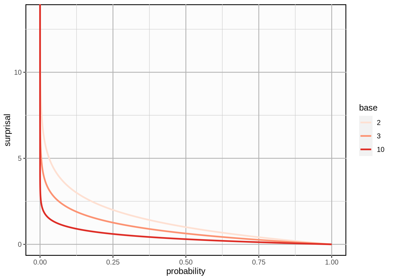
The function is strictly decreasing so surprisal inversely proportional to probability. Note that surprisal is undefined for a probability of \(0\). This is fine because we have no need to express our surprise about an event that will never occur.
A.3 Entropy
Entropy is the expected value of surprisal. This may sound odd at first. A measure that quantifies how surprised I expect to be sounds like an oxymoron. But it does make sense.
First of all, with probability, we encode our uncertainty about outcomes of a random variable. We are using all the information we have, but we know that we don’t have all the information. Thus, we know that we will be surprised about the outcome in some way because the outcome is not certain. Entropy gives us a way to quantify how surprised we expect to be about the outcome.
Entropy is given by4:
\[ H(X) := -\sum_{x \in X}{p(x)log(p(x))} \]
Useful resources on surprisal and entropy
Other terms for surprisal that you might come across are self-information and Shannon information.↩︎
You may ask yourself: Why is \(H\) the formula symbol for a metric called entropy? That’s because Shannon entropy is based on Boltzmann’s H-theorem in statistical thermodynamics. It is contested why Boltzmann called entropy \(H\), but the common conjecture is that he actually meant the greek letter Eta (\(H\)) which would make a lot more sense. There have actually been typographical analyses of his handwriting to determine whether he meant Eta, not the letter \(H\)!↩︎